Additional Factors

Precise PSF models commonly include several physical effects which may affect the PSF. They are added as amplitude factors \(a(\mathbf{s})\) and phase factors \(W(\mathbf{s})\) in the original integral over solid angles in Eq. (1):

(12)\[ \mathbf{E}(\boldsymbol{\rho}) = -\frac{\mathrm{i} fk}{2\pi}\iint\limits_{\Omega} a(\mathbf{s}) \exp{\left\{\mathrm{i} W(\mathbf{s})\right\}} \mathbf{e}_\infty(\mathbf{s}) \exp{\left\{\mathrm{i}k\mathbf{s}\cdot\boldsymbol{\rho}\right\}} \mathrm{d}\Omega.\]

Eq. (12) enables us to express these correction factors with full generality: in both vectorial and scalar models, for both Cartesian and spherical parametrizations. We present a graphical description of them in Fig. 2.

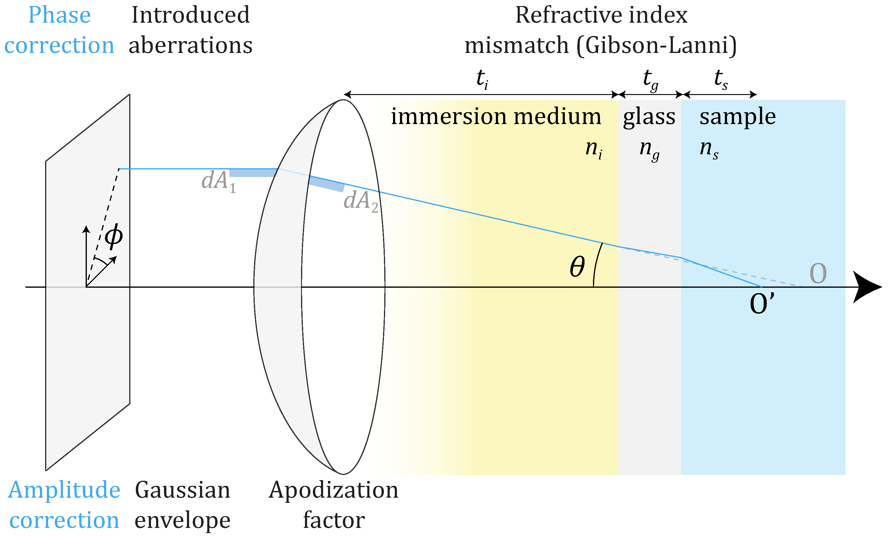
Fig. 2 Correction factors and associated physical effects. Top: phase correction factors, either introduced on the incident field or due to refraction at different planes. Bottom: amplitude correction factors, to model an incident envelope or apodization factor for energy conservation.

On the Phase

Gibson-Lanni Factor: Correction for Refractive Index Mismatch

Microscopes typically have stratified layers of different refractive indices. The biological sample is usually aqueous, on top of which we place a coverslip made of glass, and the whole sample is then put in a water or oil immersion medium to increase the numerical aperture. The microscope objectives are designed to provide aberration-free images in a specific setting with design values for refractive indices and thicknesses of the different layers. Any mismatch introduces spherical aberrations due to refraction at the different layers. These aberrations can be computed using the following formula expressed in spherical coordinates where \(\sin\theta\) is computed in the Cartesian case using \(\sin\theta = \frac{NA}{n_i}\sqrt{s_x^2+s_y^2}\):

(13)\[ W(\mathbf{s}) = \frac{2\pi}{\lambda} \left( t_s \sqrt{n_s^2 - n_i^2 \sin^2 \theta} + t_i \sqrt{n_i^2 - n_i^2 \sin^2 \theta} - t_i^* \sqrt{\left.n_i^*\right.^2 - n_i^2 \sin^2 \theta} + t_g \sqrt{n_g^2 - n_i^2 \sin^2 \theta} - t_g^* \sqrt{\left.n_g^*\right.^2 - n_i^2 \sin^2 \theta} \right)\]

where \(n_s\), \(n_i\), \(n_g\) are the refractive indices of the sample, immersion medium, and glass respectively, \(t_s\), \(t_i\), \(t_g\) are the thicknesses of the sample, immersion medium, and glass respectively, and their counterparts with stars are the design conditions.

A particular case proposed in [7] is commonly encountered: it is difficult in practice to assess the thickness of the immersion medium. Since this distance is manually tuned to obtain an optimal focus of a point emitter at depth \(t_s\) on the camera, this focusing condition gives the following relation:

(14)\[ t_i = t_s + n_i \left( -\frac{t_s}{n_s} - \frac{t_g}{n_g} + \frac{t_g^*}{n_g^*} + \frac{t_i^*}{n_i^*} \right)\]

which can be inserted in Eq. (13). This particular expression has first been derived for the spherical scalar case in [7] and extended to the spherical vectorial case in [8, 9].

Arbitrary Phase Aberrations

More general aberration models can be introduced to describe imperfections in the optical system for PSF engineering or wavefront shaping. They can be introduced experimentally via a phase mask or a spatial light modulator at the pupil plane. These aberrations are often parametrized by Zernike polynomials (a set of orthonormal polynomials defined on the pupil disk, see Fig. 3) or a direct fixed phase mask to obtain desired PSFs.

Fig. 3 Images of the first 15 Zernike polynomials. Generated using the library ZernikePy.

We write it in the most general case:

(15)\[ W(\mathbf{s}) = \sum_{k=0}^{K-1} c_k Z_k(\mathbf{s}) + W_0(\mathbf{s}).\]

Eq. (15) is composed of an inner product of the first \(K\) Zernike polynomials and their corresponding coefficients \(c_k\) and an additional term \(W_0\) which can be used to include special cases not covered by the Zernike polynomials, e.g. a vortex phase ramp that leads to a donut PSF, typically used in stimulated emission depletion microscopy.

Note that arbitrary phase aberrations described in Eq. (15) may not necessarily be axisymmetric, hence, they can only be applied to the most general, Cartesian parametrization.

On the Amplitude

Apodization Factor

The apodization factor is an amplitude correction factor to ensure energy conservation during the change of basis from cylindrical coordinates (incident field \(\mathbf{e}_\mathrm{inc}\)) to spherical coordinates (far field \(\mathbf{e}_\infty\)), which matters especially for high-NA objectives. Since areas of cross-sections are modified, the field is also rescaled accordingly. Such rescaling ensures that the differential areas \(dA_1\) on the plane and \(dA_2\) on the sphere, as shown in Fig. 2, remain consistent under the change of coordinates. The corresponding correcting factor is

\[ A(\mathbf{s}) = \sqrt{\cos\theta}\]

when going from cylindrical to spherical in the focusing configuration of Fig. 1.

Gaussian Envelop

The incident illumination can also depart from a perfect uniform plane wave. In particular, we often assume a Gaussian envelope which can be expressed as

\[ A(\mathbf{s}) = \exp\left\{-\frac{\sin^2\theta}{s_\mathrm{env}^2}\right\}\]

where the constant \(s_\mathrm{env}\) determines the size of the envelope.