Basic Theory of PSF Models

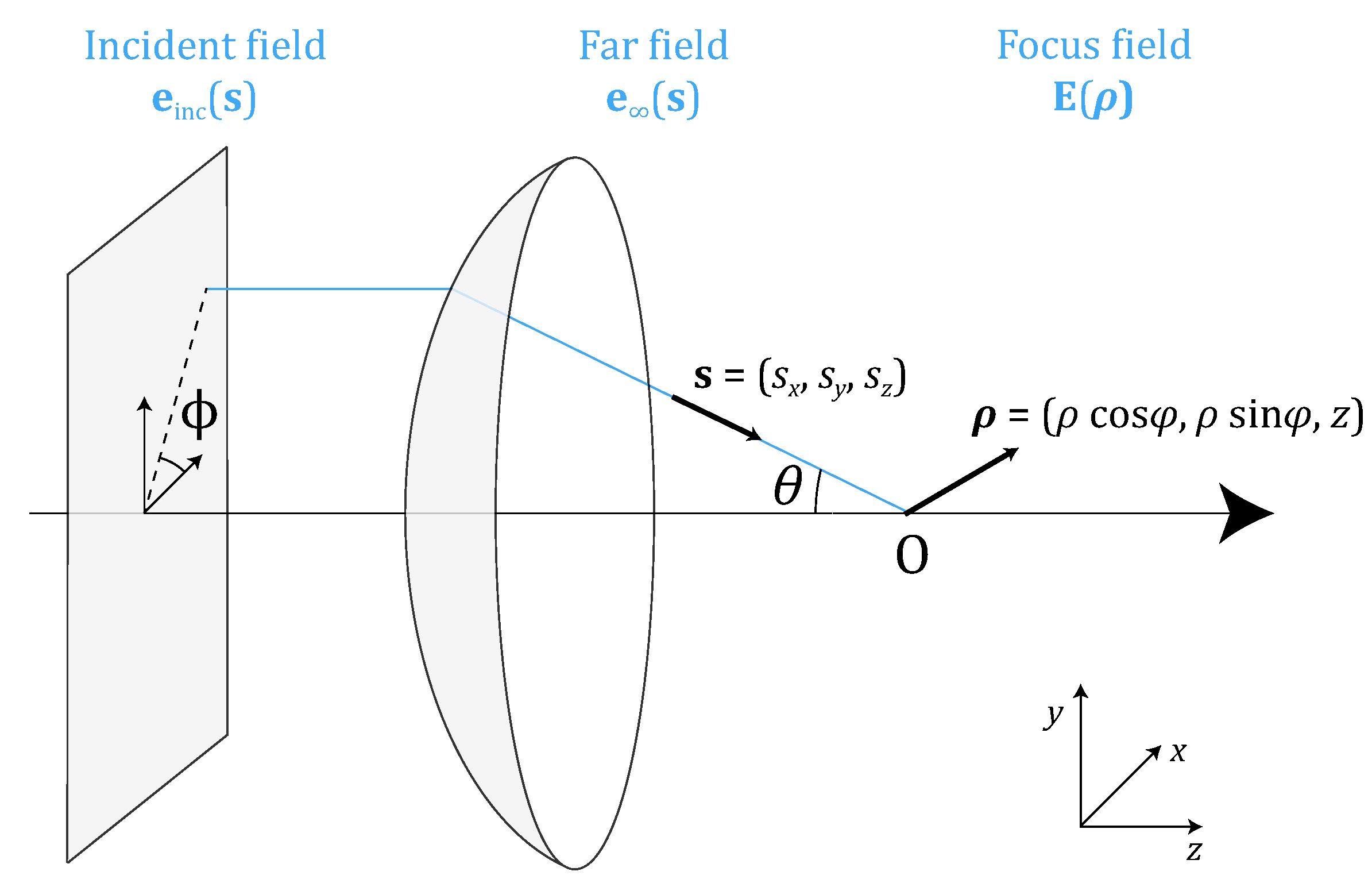
Fig. 1 Geometry of the focusing of optical fields. An incident field \(\mathbf{e}_\mathrm{inc}\) is transformed by a focusing element into a converging spherical wave \(\mathbf{e}_\infty\). These fields are parametrized by a unit vector \(\mathbf{s}\), either in Cartesian coordinates \((s_x, s_y, s_z)\) or spherical coordinates \((\theta, \phi)\). The focus field \(\mathbf{E}\) is parametrized by \(\boldsymbol{\rho} = (x, y, z)\), rewritten here to introduce cylindrical coordinates \(\rho\) and \(\phi\).

The Richards-Wolf Model: Start Point

The model introduced by Richards and Wolf [1] is the starting point that allows us to derive all the precise PSF models described in previous works.

As depicted in Fig. 1, the PSF is obtained by computing the propagation of light after going through a focusing element, typically a microscope objective or lens. The incident field \(\mathbf{e}_\mathrm{inc}(\mathbf{s})\), also called pupil function, is represented by a disk with a maximal cut-off angle defined by the NA of the imaging system. The focusing element transforms the incident field into a spherical wave, \(\mathbf{e}_\infty(\mathbf{s})\), evaluated on the Gaussian reference sphere. This corresponds to an ensemble of far fields propagating with direction \(\mathbf{s}\) all converging to the focal point \(O\). Our goal is to compute the focused electric field \(\mathbf{E}(\boldsymbol{\rho})\) around the point \(O\) for high-NA systems. Thanks to the reciprocity of light propagation, this model can also be extended to the emission of a point source to the back focal plane of a microscope objective but this is not the focus of the current study.

The focal field is given by a sum of plane waves with direction \(\mathbf{s} = (s_x,s_y,s_z)\):

(1)\[ \mathbf{E}(\boldsymbol{\rho}) = -\frac{\mathrm{i} fk}{2\pi}\iint\limits_{\Omega}\mathbf{e}_\infty(\mathbf{s}) \exp{\left\{\mathrm{i}k\mathbf{s}\cdot\boldsymbol{\rho}\right\}} \mathrm{d}\Omega\]

where \(\boldsymbol{\rho} = (x,y,z) = (\rho\cos\varphi, \rho\sin\varphi,z)\) is the position vector in the focal region of the lens, \(\mathbf{s} = (s_x,s_y,s_z) = (\sin\theta \cos\phi, \sin\theta \sin\phi, \cos\theta)\) is a unit vector describing the direction of an incoming ray, \(f\) is the focal length of the lens, \(k = \frac{2\pi n}{\lambda}\) is the wavenumber, \(\lambda\) is the wavelength, \(n\) is the refractive index of the propagation medium, and \(\mathbf{e}_\infty(\mathbf{s})\) describes the field distribution on the Gaussian reference sphere. We integrate over set \(\Omega\) of solid angles defined on a region \(s_x^2 + s_y^2 \leq s_\mathrm{max}^2\), where \(s_\mathrm{max} = \frac{\mathrm{NA}}{n_i}\) is the cut-off determined by the NA. The angle \(\theta\) is defined in the immersion medium. Correction factors are typically introduced in this expression but we will first describe the different classes of models based on this simplified concise equation.

Scalar Models

It is common to employ a scalar approximation to simplify calculations, especially in low-NA scenarios. In this case, the far field is equal to the incident field, i.e. \(e_\infty(\mathbf{s}) = e_\mathrm{inc}(\mathbf{s})\) and the focal field is given by:

(2)\[ E(\boldsymbol{\rho}) = -\frac{\mathrm{i} fk}{2\pi}\iint\limits_{\Omega}e_\infty(s_x,s_y) \exp{\left\{\mathrm{i}k\mathbf{s}\cdot\boldsymbol{\rho}\right\}} \mathrm{d}\Omega.\]

This expression involves a two-dimensional integral over the pupil disk. Two possible parametrizations that yield the two classes of models described previously can be employed.

Cartesian parameterization

The Cartesian parametrization utilizes both \(s_x\) and \(s_y\) coordinates with \(\mathrm{d}\Omega = \mathrm{d}s_x \mathrm{d}s_y / s_z\), resulting in:

(3)\[ E(\boldsymbol{\rho}) = -\frac{\mathrm{i} fk}{2\pi}\iint\limits_{s_x^2 + s_y^2 \leq s_{\max}^2} \frac{e_\infty(s_x,s_y)}{s_z} \exp{\left\{\mathrm{i}ks_z z\right\}} \exp{\left\{\mathrm{i} k (s_x x + s_y y)\right\}} \mathrm{d}s_x \mathrm{d}s_y.\]

In this form, the focused field at a given transverse plane is given by the 2D inverse Fourier transform of \((e_\infty(s_x,s_y)\exp{\left\{\mathrm{i} k s_z z\right\}} / s_z)\), where \(s_z = \sqrt{1-s_x^2-s_y^2}\). Thus, the Cartesian parametrization of the Richards-Wolf integral leverages the speed and efficiency of the Fast Fourier Transform (FFT) algorithm.

Spherical parameterization

Alternatively, the spherical approach parametrizes the problem with two angles \(\theta \in [0, \theta_{\max}]\) (the maximum angle \(\theta_{\max}\) is determined by the NA) and \(\phi \in [0, 2\pi]\), as depicted in Fig. 1. With \(\boldsymbol{\rho} = (x,y,z) = (\rho\cos\varphi, \rho\sin\varphi,z)\) and \(\mathrm{d}\Omega = \sin\theta \mathrm{d}\theta \mathrm{d}\phi\), the field in the focal region can be rewritten as:

(4)\[ E(\boldsymbol{\rho}) = -\frac{\mathrm{i} fk}{2\pi} \int_0^{\theta_{\max}} \mathrm{d}\theta \int_0^{2\pi} \mathrm{d}\phi e_\infty(\theta,\phi) \exp{\left\{\mathrm{i}k\rho\sin\theta\cos(\phi-\varphi)\right\}} \exp{\left\{\mathrm{i}kz\cos\theta\right\}} \sin\theta.\]

Eq. (4) can be further simplified if one assumes that the pupil function is axisymmetric (rotational invariant), i.e. \(e_\infty(\theta, \phi) = e_\infty(\theta)\). In this case the integral over \(\phi\) in Eq. (4) can be computed explicitly using the Bessel function \(J_0\).

(5)\[ E(\boldsymbol{\rho}) = -\mathrm{i} fk \int_0^{\theta_{\max}} \mathrm{d}\theta e_\infty(\theta) J_0(k \rho \sin \theta) \exp{\left\{\mathrm{i}kz\cos\theta\right\}} \sin\theta.\]

The spherical parametrization often uses the following identities where \(J_n\) is the Bessel function of \(n\)th-order of the first kind:

\[ \int_{0}^{2\pi} \cos(n\phi) \exp{\left\{\mathrm{i} x \cos(\phi-\varphi)\right\}}\mathrm{d}\phi = 2\pi(\mathrm{i})^n J_n(x)\cos(n\varphi)\]

\[ \int_{0}^{2\pi} \sin(n\phi) \exp{\left\{\mathrm{i} x \cos(\phi-\varphi)\right\}}\mathrm{d}\phi = 2\pi(\mathrm{i})^n J_n(x)\sin(n\varphi)\]

Defocus is included in these models using the defocus phase factor \(\exp{\left\{\mathrm{i}k s_z z\right\}} = \exp{\left\{\mathrm{i}kz \cos\theta\right\}}\) where \(z\) is the defocus distance. This expression, also known as angular spectrum propagation [12], accurately models the propagation of electric field in a homogeneous medium.

Vectorial Models

As the electric field is a vectorial quantity, vectorial propagation models are necessary to accurately account for the propagation and crosstalk between the different components of the vector field. Employing these precise vectorial models is crucial for high-NA systems in which case the need to consider high angles arises.

In the vectorial model, the far field \(\mathbf{e}_\infty(\mathbf{s})\) now has a more complex dependence on the incident field \(\mathbf{e}_\mathrm{inc}(\mathbf{s})\) as we need to perform the basis change from a cylindrical to a spherical coordinate system:

(6)\[\begin{split} \mathbf{e}_\infty(\theta,\phi) = \begin{bmatrix} q_s(1-\cos2\phi) + q_p(1+\cos2\phi)\cos\theta \\ (-q_s+q_p\cos\theta)\sin2\phi \\ -2 q_p \cos\phi \sin\theta \end{bmatrix} \frac{e_\mathrm{inc}^x(\theta,\phi)}{2} + \begin{bmatrix} (-q_s+q_p\cos\theta)\sin2\phi \\ q_s (1+\cos2\phi) + q_p (1-\cos2\phi) \cos\theta \\ - 2 q_p \sin\phi \sin\theta \end{bmatrix} \frac{e_\mathrm{inc}^y(\theta,\phi)}{2}\end{split}\]

where \(\mathbf{e}_\mathrm{inc} = [e_\mathrm{inc}^x, e_\mathrm{inc}^y, 0]\). Fresnel transmission coefficients \(q_s\) and \(q_p\) have been introduced to account for partial reflection at interfaces, which depend on the polarization state and incidence angle. For each of the \(s\) and \(p\) polarizations, they correspond to the product of all transmission coefficients for each interface from medium \(j\) to \(j+1\):

\[ q_s^{j} = \frac{2 n_j \cos{\theta_j}}{n_j\cos\theta_j+n_{j+1}\cos{\theta_{j+1}}},\]

\[ q_p^{j} = \frac{2 n_j \cos{\theta_j}}{n_{j+1}\cos\theta_j+n_{j}\cos{\theta_{j+1}}}.\]

Cartesian Parameterization

The Cartesian parametrization of the vectorial model consists of the following integral:

(7)\[ \mathbf{E}(\boldsymbol{\rho}) = -\frac{\mathrm{i} fk}{2\pi}\iint\limits_{s_x^2+s_y^2 \leq s_{\max}^2}\frac{\mathbf{e}_\infty(s_x, s_y)}{s_z}\exp{\left\{\mathrm{i}k s_z z\right\}}\exp{\left\{\mathrm{i}k(s_x x + s_y y)\right\}} \mathrm{d}s_x \mathrm{d}s_y,\]

which essentially boils down to computing the inverse Fourier Transform of \((\mathbf{e}_\infty(s_x, s_y) \exp{\left\{\mathrm{i}k s_z z\right\}}/s_z)\), similar to the scalar case.

Spherical Parameterization

Using coordinate transformations similar to the scalar case, we can derive the spherical parametrization of the field in the focal region:

(8)\[ \mathbf{E}(\boldsymbol{\rho}) = -\frac{\mathrm{i} fk}{2\pi}\int_0^{\theta_{\max}} \mathrm{d}\theta \int_0^{2\pi} \mathrm{d}\phi\,\mathbf{e}_\infty(\theta,\phi) \exp{\left\{\mathrm{i}k\rho\sin\theta\cos(\phi-\varphi)\right\}} \exp{\left\{\mathrm{i}kz\cos\theta\right\}} \sin\theta.\]

Inserting (6) into (8) and using the axisymmetric assumption of the incident field, we can obtain a simplified expression for the focal field as follows:

\[\begin{split} \mathbf{E}(\boldsymbol{\rho}) = - \frac{\mathrm{i} fk}{2} \left[ \begin{array}{c} [I_{0}^x - I_{2}^x\cos2\varphi] - I_{2}^y\sin2\varphi\\ - I_{2}^x\sin2\varphi + [I_{0}^y + I_{2}^y\cos2\varphi]\\ -2\mathrm{i}I_{1}^x\cos\varphi -2\mathrm{i}I_{1}^y\sin\varphi \end{array} \right]\end{split}\]

where

(9)\[ I_{0}^a (\rho,z) = \int_0^{\theta_{\max}} e_\mathrm{inc}^a(\theta)\sin\theta (\cos\theta+1) J_0(k\rho\sin\theta)\exp{\left\{\mathrm{i}kz\cos\theta\right\}}\mathrm{d}\theta\]

(10)\[ I_{1}^a (\rho,z)= \int_0^{\theta_{\max}} e_\mathrm{inc}^a(\theta)\sin^2\theta J_1(k\rho\sin\theta)\exp{\left\{\mathrm{i}kz\cos\theta\right\}}\mathrm{d}\theta\]

(11)\[ I_{2}^a (\rho,z) = \int_0^{\theta_{\max}} e_\mathrm{inc}^a(\theta)\sin\theta (\cos\theta-1) J_2(k\rho\sin\theta)\exp{\left\{\mathrm{i}kz\cos\theta\right\}}\mathrm{d}\theta\]

with \(a\in\{x,y\}\) and \(\mathbf{e}_\mathrm{inc}(\theta) = [e_\mathrm{inc}^x(\theta), e_\mathrm{inc}^y(\theta),0]\).